Attractor Maps and Function Approximation
Revision 3 2024-08-31
Revision 2 2024-04-05
Revision 1 2022-08-24
'Maps' are commonly encountered in programming and often mean a look-up table; an input maps to an output. If an attractor functionality is added to the front of the map — such that if a key is provided which does not have an entry in the map, the closest existing key (according to some distance function) is found and that key is used instead — it creates an 'attractor-map', functioning as though the keys in the map have a kind of gravity which pulls nearby inputs towards them. This is useful for a variety of purposes.
Implementation
Perl already has maps in the form of hashes which are part of the language. The attractor functionality can be easily implemented using various list processing functions, and the code ends up being terse. In this code, to create an attractor map, the sub "amap_factory" is called which returns the attractor map in the form of an anonymous sub performing a closure around a hash (for the mapping functionality), the distance function used, and a distance threshold parameter. The distance function used depends on the application.
Examples
Due to their attractor behaviour, attractor maps are often useful for seeing through noise in an input signal.
Spelling Correction
The code below shows an attractor map used to correct spelling mistakes. The attractor map is seeded with known correct spellings and mispellings. The attractor functionality allows it to correct other spelling mistakes. A measure of string edit distance is used as the distance metric, specifically the Damerau Levenshtein edit distance.
use v5.16;

package attractor_map;
use List::Util qw(reduce shuffle);

sub amap_factory {

	my ($dist_func, $threshold) = @_;

	$threshold //= 0;
	my %lookup_table; 		# the hash used for look up

	return sub {

		my ($input, $output) = @_;

		# if we are passed an output, then we are 'training' the A-map
		$lookup_table{$input} = $output if defined $output;

		# perform the lookup
		return $lookup_table{$input} if exists $lookup_table{$input};	# direct hit!

		# otherwise find nearest existing key within distance threshold and return that output (attractor behaviour)
		my $nearest =										        # 6. $nearest = [ distance, key ]
			reduce { $a->[0] < $b->[0] ? $a : $b }			        # 5. find the closest (minimum distance) out of those
			shuffle											        # 4. randomize order to give random answer in case of contested minimum
			grep { ($_->[0] <= $threshold) && defined($_->[0]) } 	# 3. disregard those keys beyond distance threshold
			map { [ $dist_func->($_, $input), $_ ] } 				# 2. compute distance from input key, put this distance beside the key
			keys %lookup_table;										# 1. for all existing hash keys

		# if we've found a hash key then perform the lookup, otherwise return undef
		return defined $nearest ? $lookup_table{ $nearest->[1] } : undef;
	}
}

package main;
use Text::Levenshtein::Damerau::XS 'xs_edistance';
# Since we are correcting spelling mistakes, use a measure of string edit distance as the distance function.
my $aMap = attractor_map::amap_factory( \&xs_edistance, 4 );

# seed with correct word spellings
$aMap->('apparent', 'apparent');
$aMap->('indispensable', 'indispensable');
$aMap->('liaison', 'liaison');
$aMap->('millennium', 'millennium');

# add some known misspellings if desired
$aMap->('indispensible', 'indispensable');
$aMap->('milennium', 'millennium');

# have some text with spelling mistakes
# spelling mistakes which have not been trained for will be dealt with by the 'attractor' behaviour
my $misspelled = q{It was apparrent that the liason was indispensible at the milenium games};

say "Correct spelling.\n";
say "Input =\n$misspelled\n\n";

# fix the longer words
my @corrected;
foreach my $word (split(/\s/, $misspelled)) {

	if ( length($word) > 5 ) {

		push @corrected, $aMap->($word);
	}
	else {
		push @corrected, $word;
	}
}

say "Output =\n", join(" ", @corrected);

exit;
Symbol Recognition
Although Perl hashes are one-dimensional strings, 2D (and higher) data arrays can be collapsed, encoded to string format and fed into the lookup table. In some cases the distance function might need to know about the higher dimensionality, but in the example below it's not necessary. Small 2D stringified bitmaps representing the shape of characters of various kinds are added to the attractor map such that they map to the text character they represent (like in OCR). The attractor functionality permits characters to be recognised even when bitmaps with some noise are presented.
use v5.16;

package distance_measures;
use Bit::Vector;
sub hamming_bitwise {

	my ( $key1, $key2 ) = @_;

	my ( $key1_len, $key2_len ) = ( length($key1), length($key2) );

	return undef unless ($key1_len > 0) && ($key1_len == $key2_len);

	my $vec1 = Bit::Vector->new_Bin( $key1_len, $key1 );
	my $vec2 = Bit::Vector->new_Bin( $key2_len, $key2 );

	$vec1->Xor( $vec1, $vec2 );
	my $norm = $vec1->Norm();

	return $norm;
}

package attractor_map;
use List::Util qw(reduce shuffle);

sub amap_factory {

	my ($dist_func, $threshold) = @_;

	$threshold //= 0;
	my %lookup_table; 		# the hash used for look up

	return sub {

		my ($input, $output) = @_;

		# if we are passed an output, then we are 'training' the A-map
		$lookup_table{$input} = $output if defined $output;

		# perform the lookup
		return $lookup_table{$input} if exists $lookup_table{$input};	# direct hit!

		# otherwise find nearest existing key within distance threshold and return that output (attractor behaviour)
		my $nearest =										        # 6. $nearest = [ distance, key ]
			reduce { $a->[0] < $b->[0] ? $a : $b }			        # 5. find the closest (minimum distance) out of those
			shuffle											        # 4. randomize order to give random answer in case of contested minimum
			grep { ($_->[0] <= $threshold) && defined($_->[0]) } 	# 3. disregard those keys beyond distance threshold
			map { [ $dist_func->($_, $input), $_ ] } 				# 2. compute distance from input key, put this distance beside the key
			keys %lookup_table;										# 1. for all existing hash keys

		# if we've found a hash key then perform the lookup, otherwise return undef
		return defined $nearest ? $lookup_table{ $nearest->[1] } : undef;
	}
}

package main;

# create an attractor map working off bit distance
my $aMap = attractor_map::amap_factory( \&distance_measures::hamming_bitwise, 6 );

# flattened 7 by 7 bitmap icons representing some basic maths symbols
(my $plus_symbol = q{
0001000
0001000
0001000
1111111
0001000
0001000
0001000
}) =~ s/\n//gimsx;

(my $X_symbol = q{
1000001
0100010
0010100
0001000
0010100
0100010
1000001
}) =~ s/\n//gimsx;

(my $minus_symbol = q{
0000000
0000000
0000000
1111111
0000000
0000000
0000000
}) =~ s/\n//gimsx;

(my $equals_symbol = q{
0000000
0000000
1111111
0000000
1111111
0000000
0000000
}) =~ s/\n//gimsx;

(my $exclam_symbol = q{
0001000
0001000
0001000
0001000
0001000
0000000
0001000
}) =~ s/\n//gimsx;


# 'train' the attractor map to recognise the symbols
$aMap->($plus_symbol, '+');
$aMap->($X_symbol, 'X');
$aMap->($minus_symbol, '-');
$aMap->($equals_symbol, '=');
$aMap->($exclam_symbol, '!');

# define some bitmaps with added noise
(my $noisy_plus = q{
1001000
0001010
0001000
1111111
0001100
0011000
0001000
}) =~ s/\n//gimsx;

(my $noisy_equals = q{
0000010
0000100
1111001
0000000
1111111
0000000
0100000
}) =~ s/\n//gimsx;

# see if the attractor map can recognise the noisy symbols

if ( $aMap->($plus_symbol) eq '+' ) {
	say "Recognised plus (no noise)";
}
else {
	say "Did not recognise plus! (no noise)";
}

if ( $aMap->($noisy_plus) eq '+' ) {
	say "Recognised plus (with noise)";
}
else {
	say "Did not recognise plus! (with noise)";
}

if ( $aMap->($equals_symbol) eq '=' ) {
	say "Recognised equals (no noise)";
}
else {
	say "Did not recognise equals! (no noise)";
}

if ( $aMap->($noisy_equals) eq '=' ) {
	say "Recognised equals (with noise)";
}
else {
	say "Did not recognise equals! (with noise)";
}

exit;
Function Approximation
Up to now the attractor-maps have been dealing with one input parameter. However, it is certainly possible to create attractor-maps which take in multiple parameters; the distance function simply has to work in a higher-dimensional space (and, in Perl, the inputted variables have to be able to be combined and stringified into a hash key for lookup). This is useful for function approximation, e.g. f(x, y, z) → u, but f isn't fully known, however there are samples.
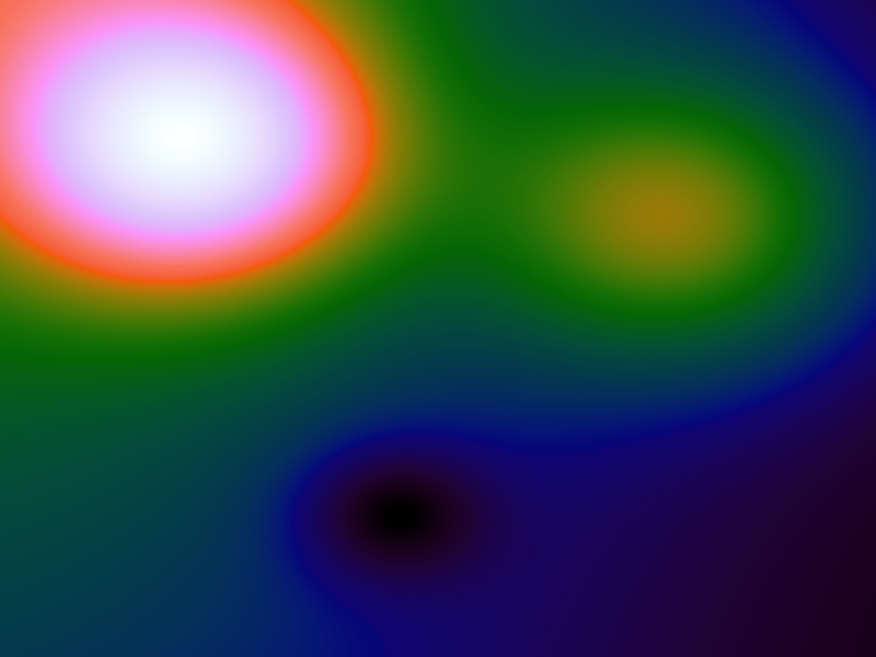
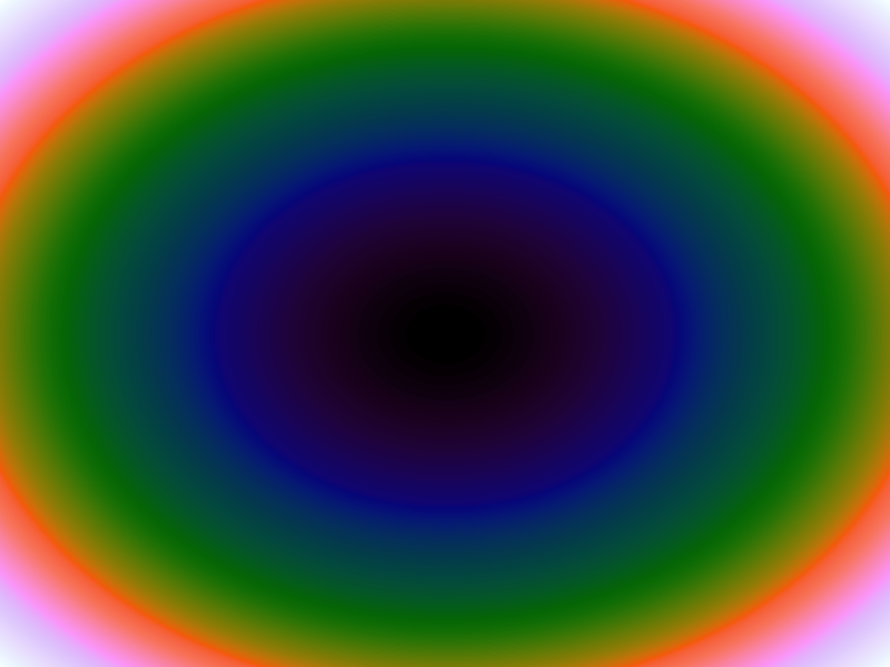
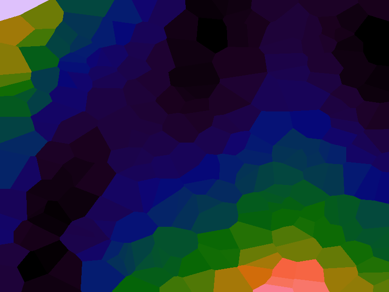
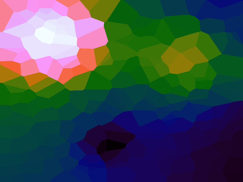
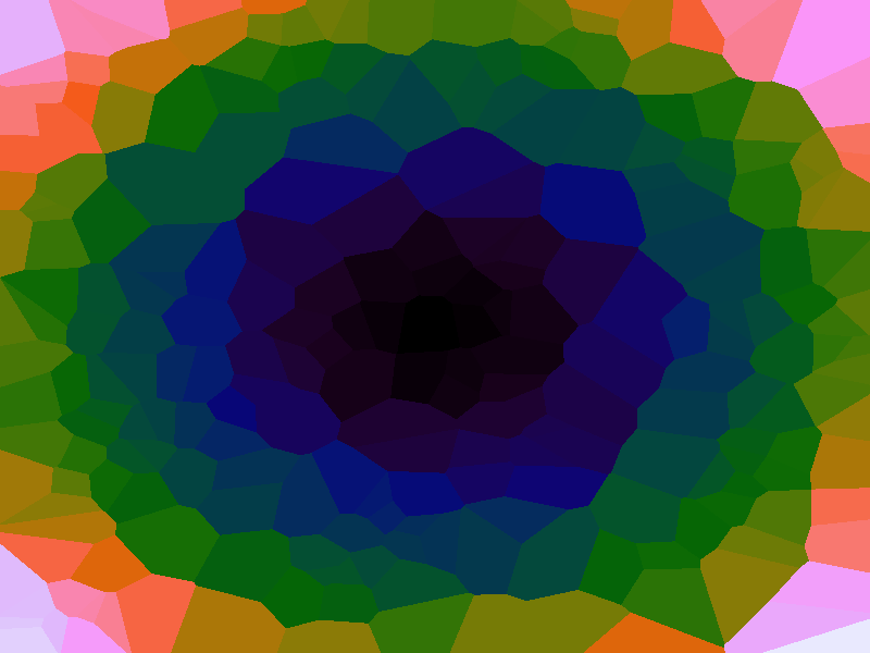
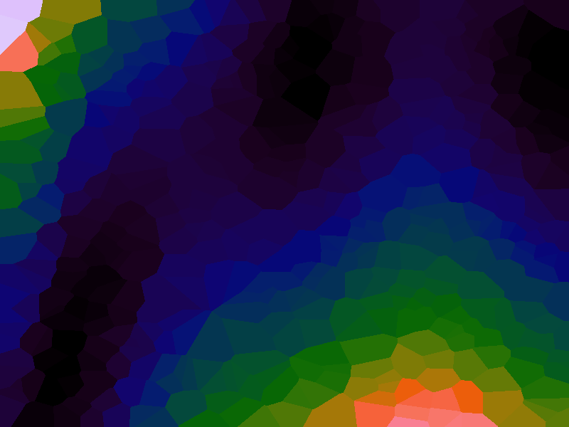
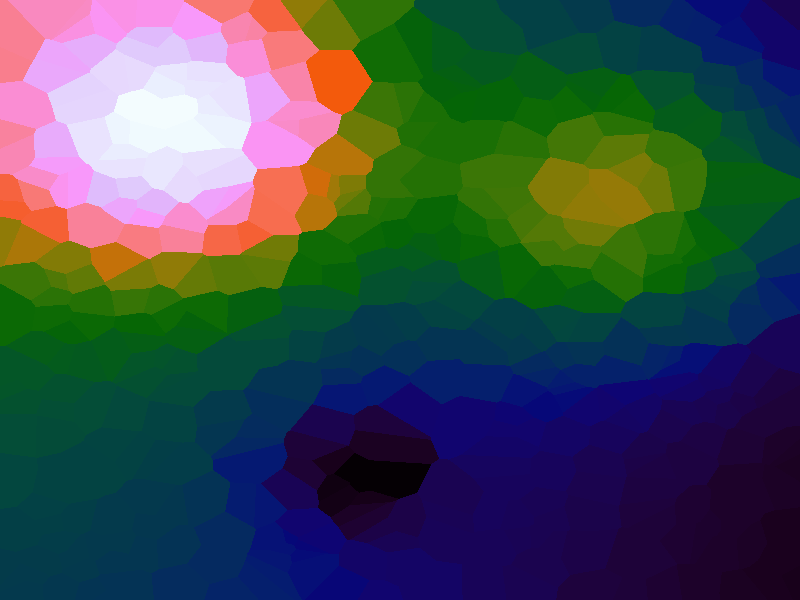
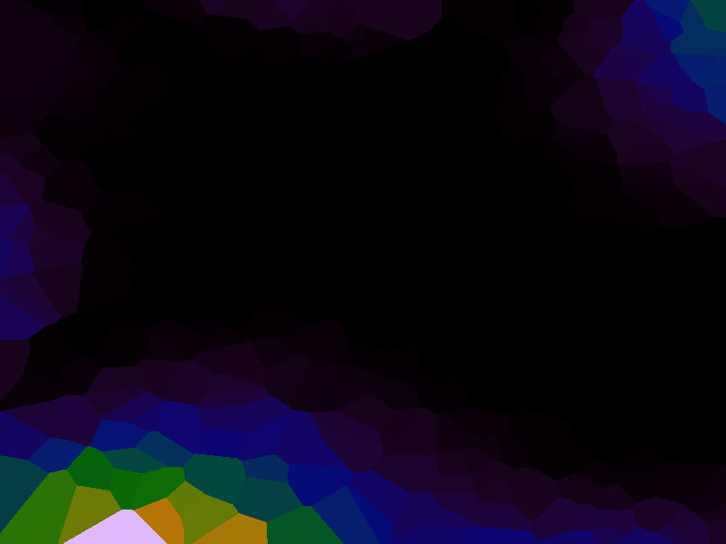
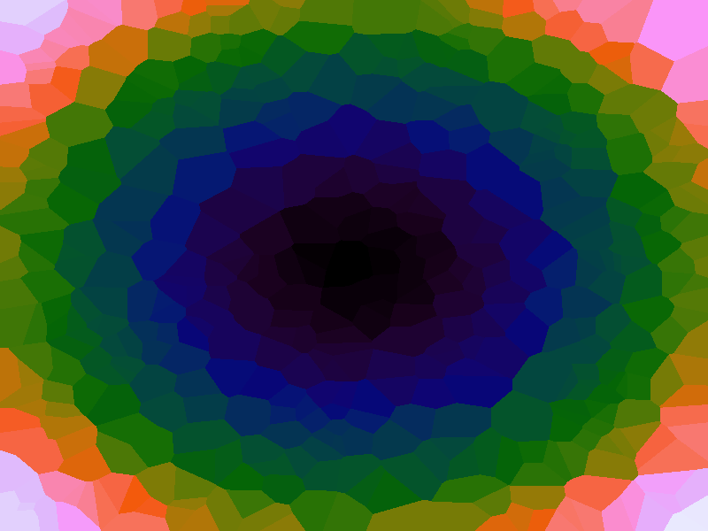
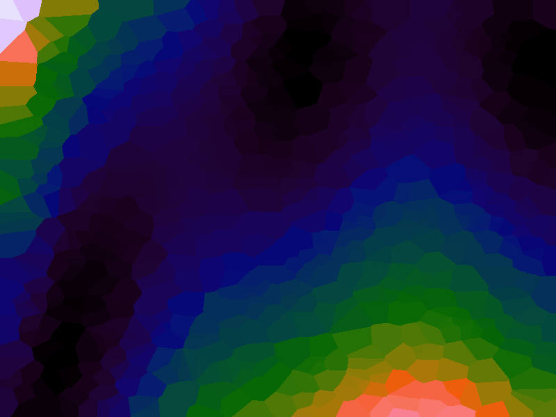
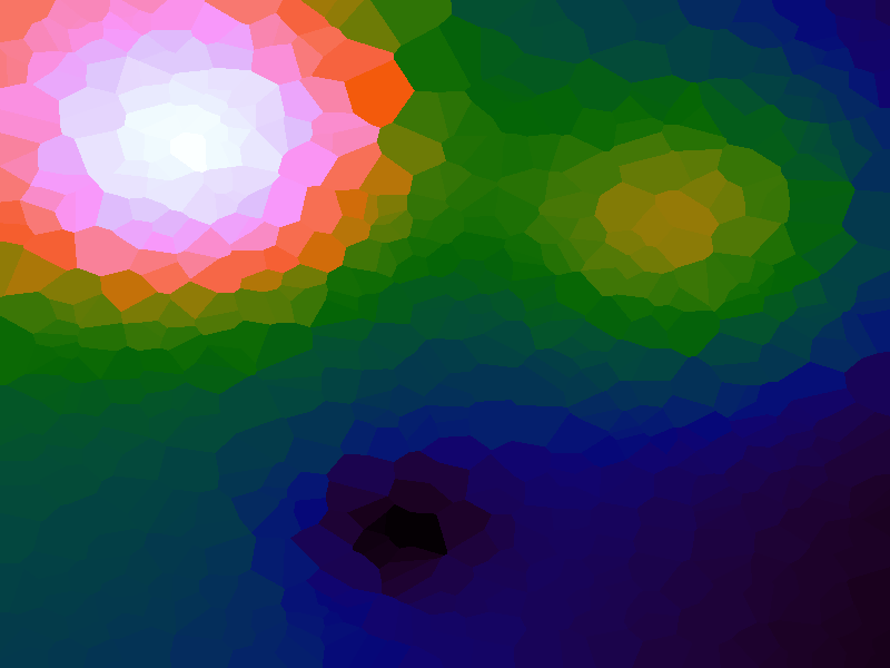
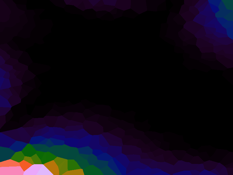
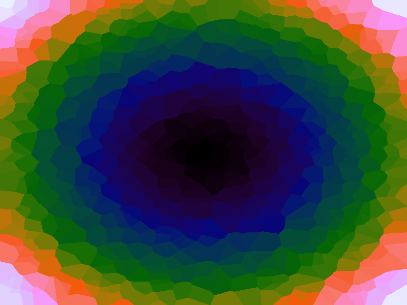
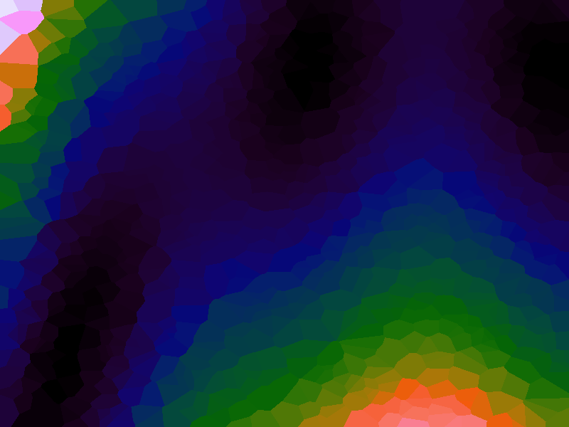
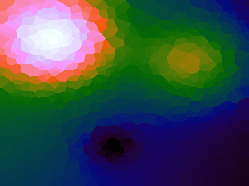
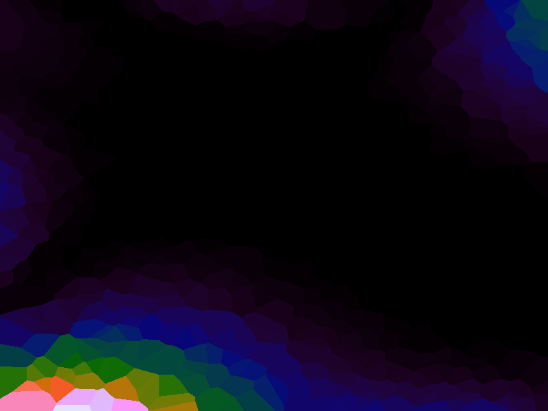
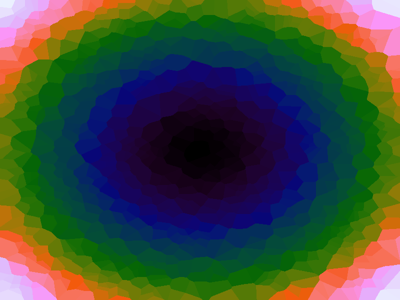
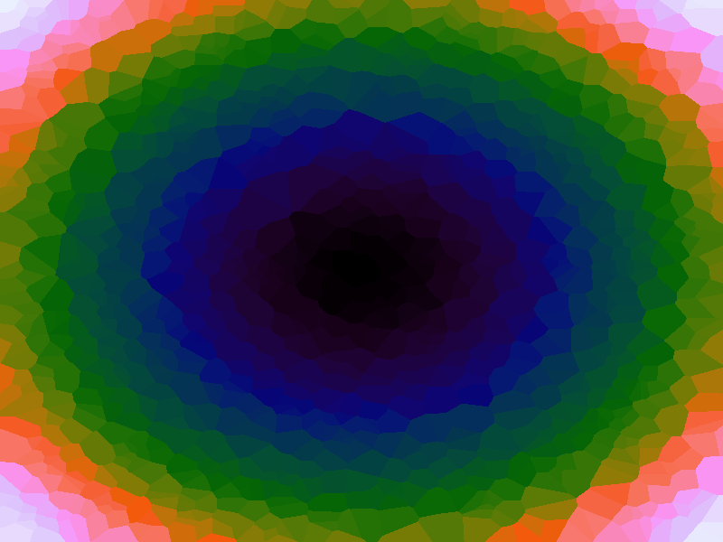
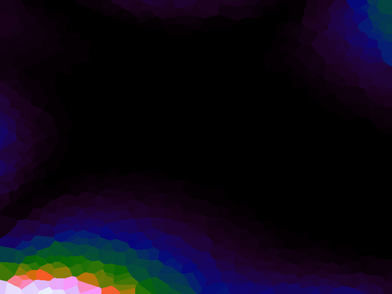
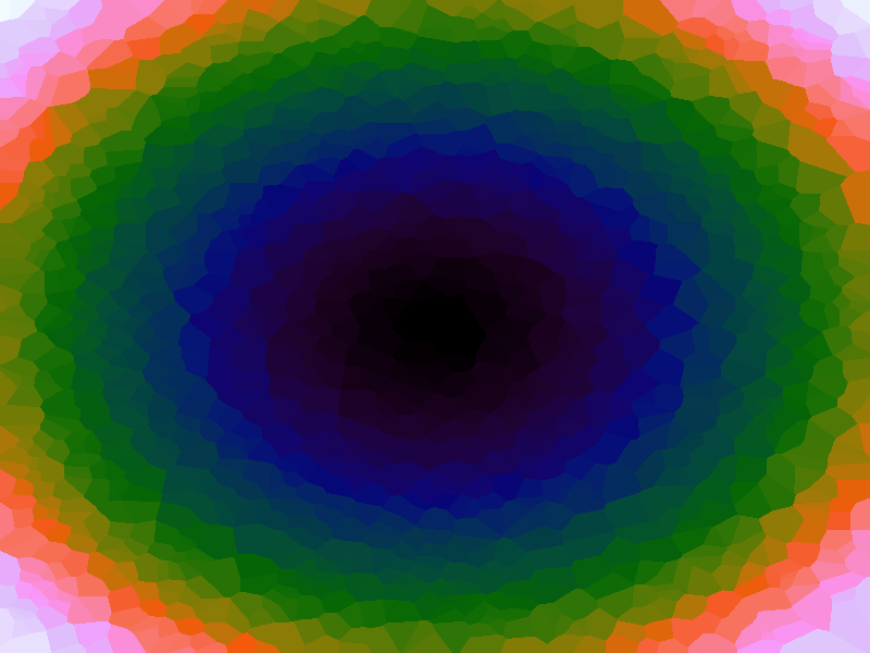
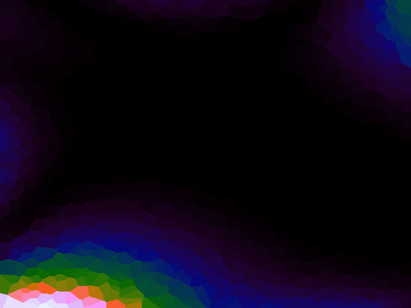
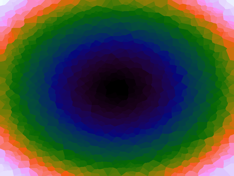
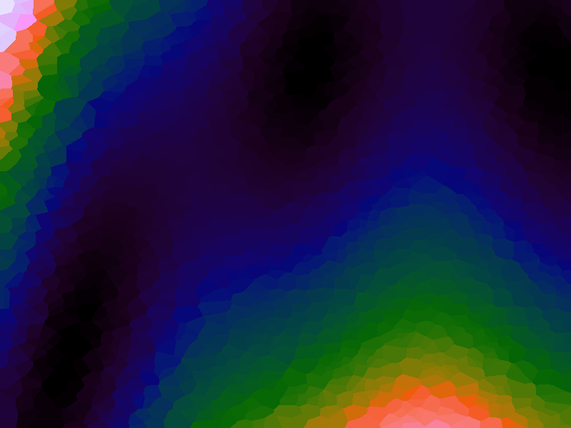
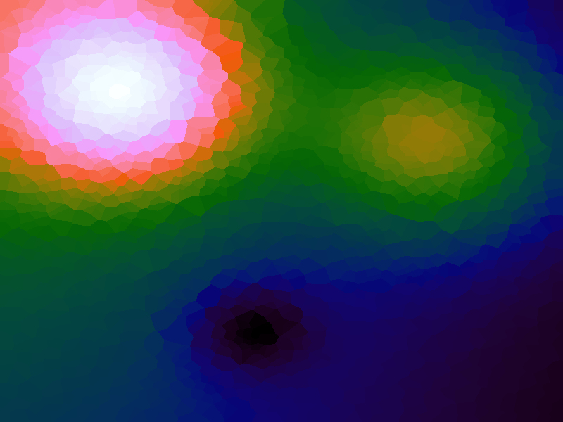
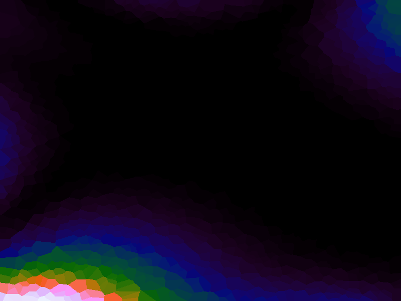
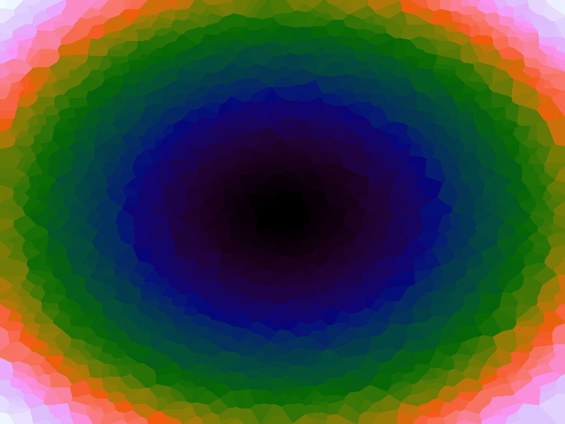
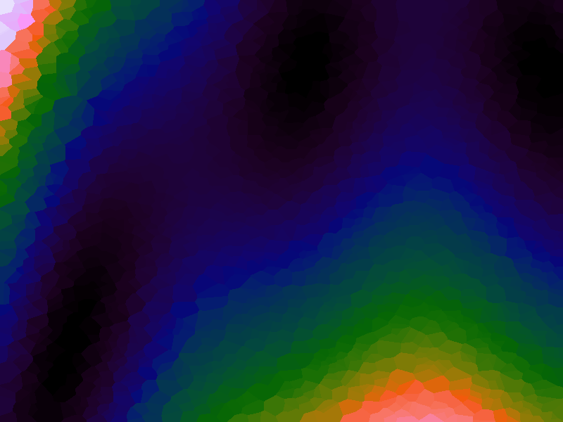
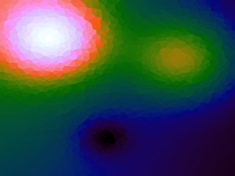
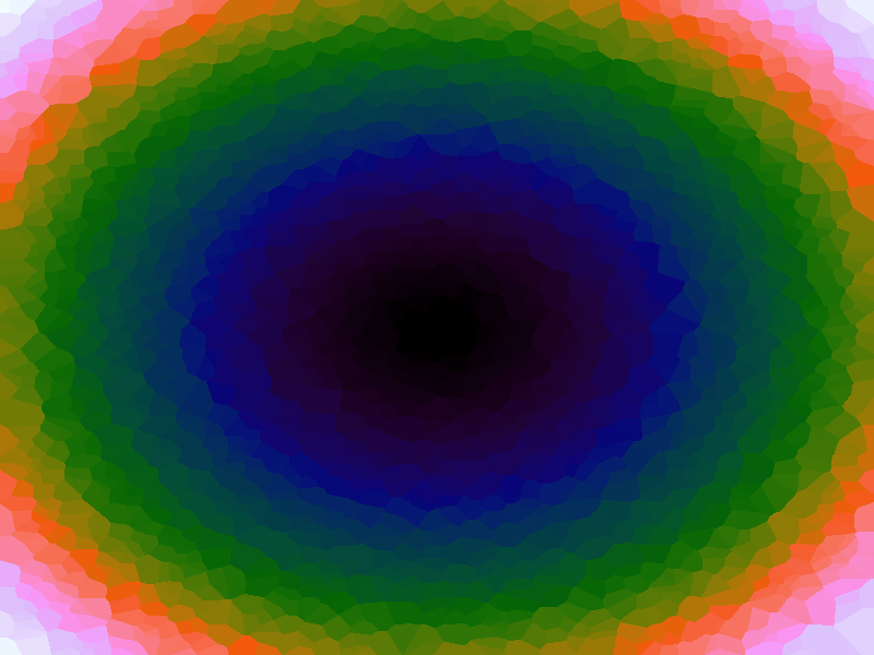
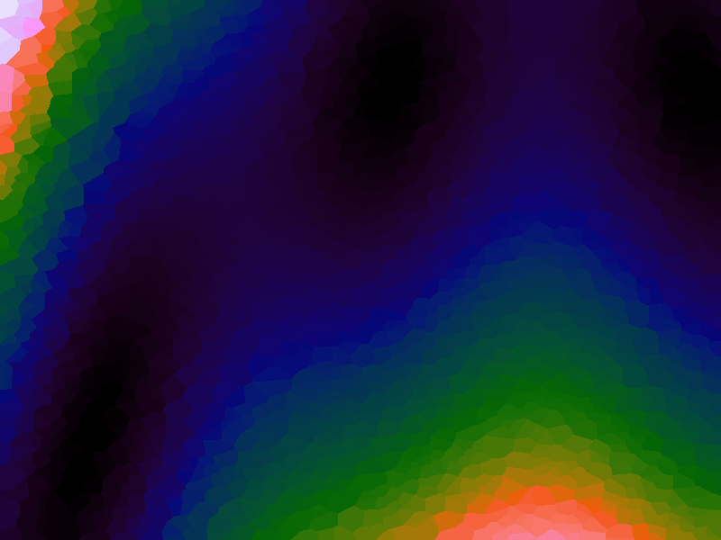
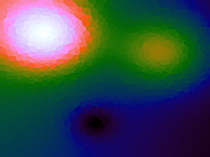
A function can be represented precisely as an equation of its input variables, but also approximately by sampling it at regular or irregular intervals and then interpolating the outputs to come up with an approximate output when presented with an arbitrary input. In this way the attractor-map arrangement can be used for function approximation, specifically function approximation through nearest-neighbour interpolation. Table 1 below demonstrates this using a variety of widely-used functions (which can be found here).
The functions are of two variables, so the usual 2D Euclidian distance metric is used as the distance function. Instead of visualising using a 3D graph, a heatmap approach is used, as this better shows the nearest-neighbour approximation (brighter colours indicate a higher output value). The attractor map is seeded with an increasing number of random sample data points taken from within the typically-used range of each function, and as expected, as the number of sample points increases, the accuracy of the approximation also increases (heatmaps were found here).
Some functions, such as the Ackley, are very difficult to approximate, particularly with nearest-neighbour. However, there is rarely a need to try to approximate a function where an equation is already known. Usually this kind of approach is taken where the function is not known (or might not exist) but there are some empirical measurements. For example, heightmap data for a geographical terrain, and an approximation for a height at an arbitrary grid location is required. The functions below are used purely for demonstration.
| Function | Ackley | Branin | Franke's | Goldstein-Price | Sphere |
|---|---|---|---|---|---|
| Original | 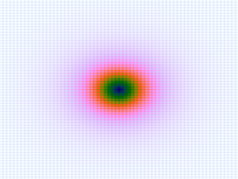 |
 |
 |
 |
 |
| 250 points | 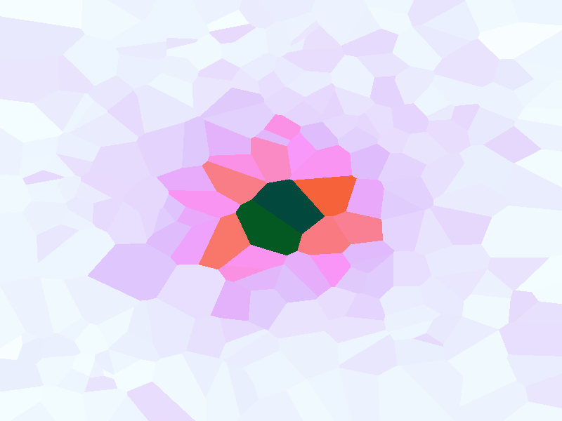 |
 |
 |
 |
 |
| 500 points | 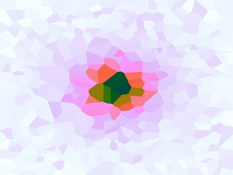 |
 |
 |
 |
 |
| 750 points | 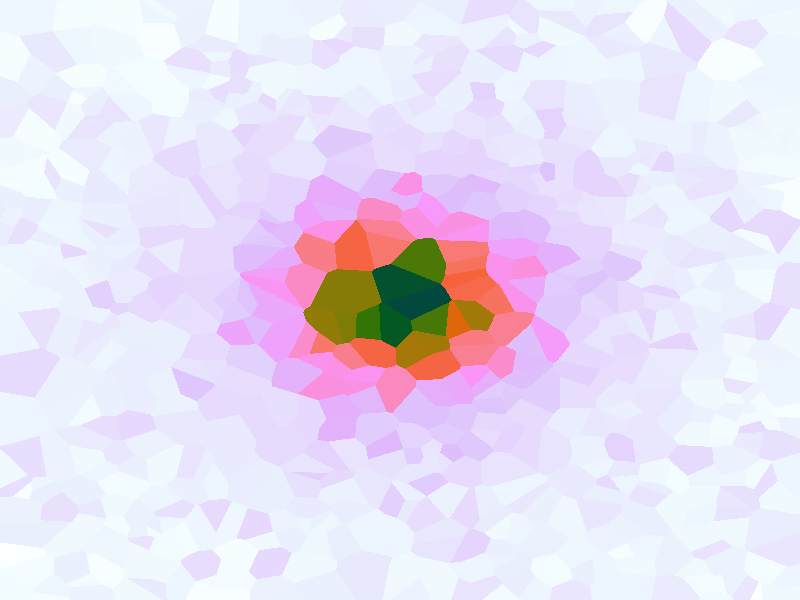 |
 |
 |
 |
 |
| 1000 points | 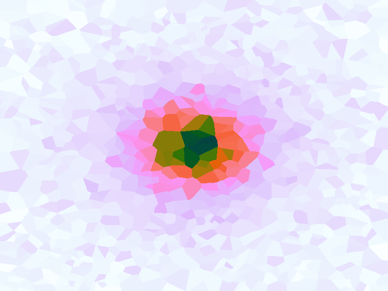 |
 |
 |
 |
 |
| 1250 points | 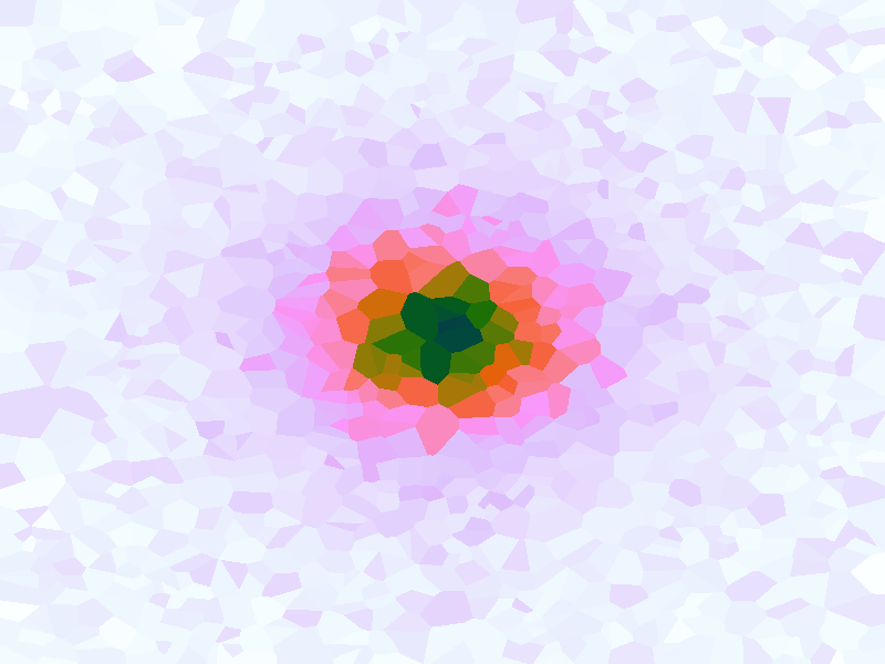 |
 |
 |
 |
 |
| 1500 points | 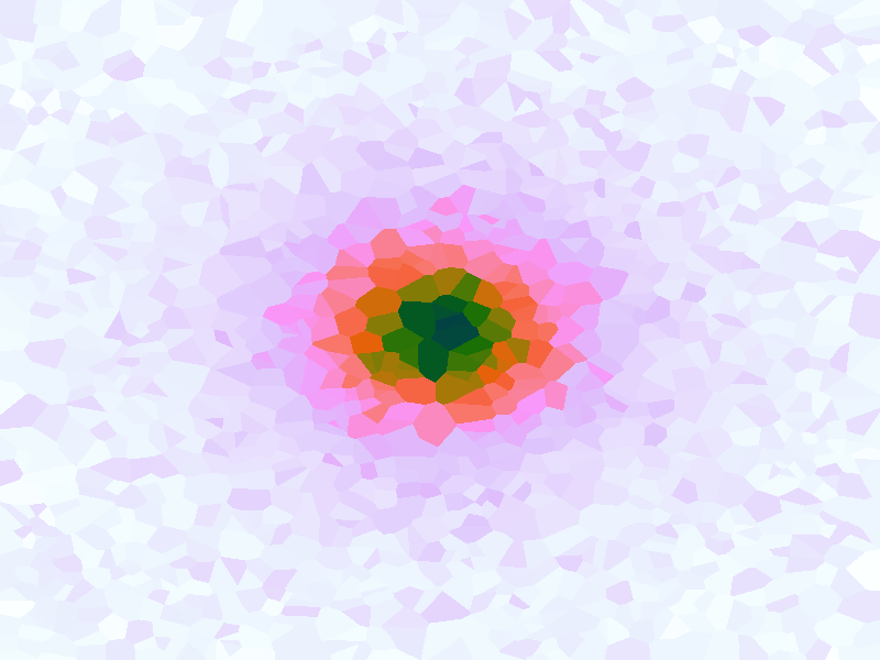 |
 |
 |
 |
 |
| 1750 points | 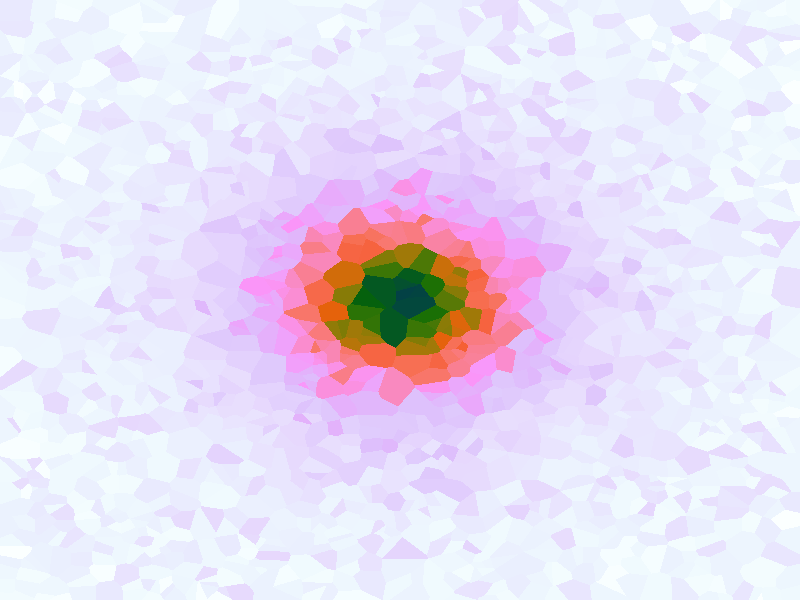 |
 |
 |
 |
 |
| 2000 points | 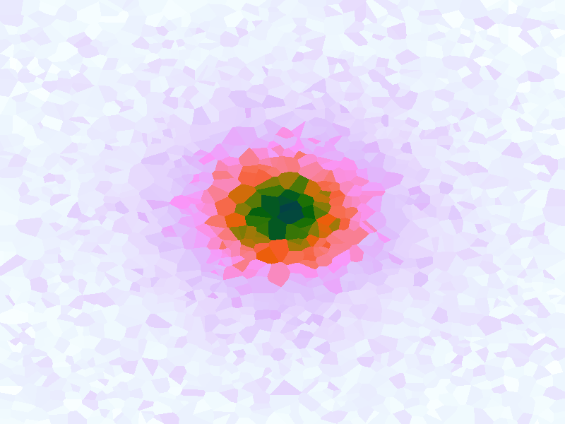 |
 |
 |
 |
 |
| 2250 points | 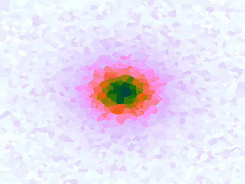 |
 |
 |
 |
 |
| 2500 points | 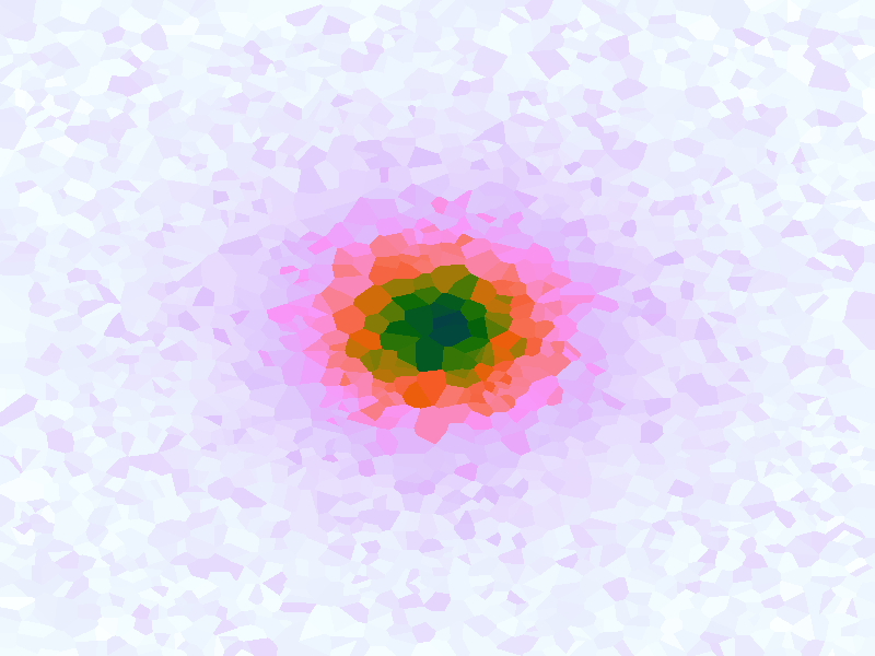 |
 |
 |
 |
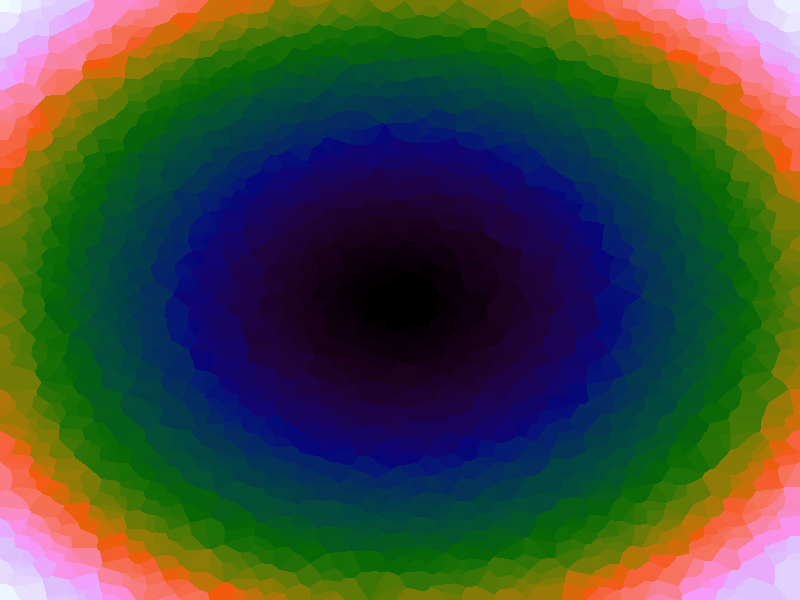 |
Table 1. Comparison of different approximated functions with increasing number of sample points.
Optimisations
When the attractor map is fed with thousands of sampled data points, performing thousands of lookups can become slow. There are two obvious speed-ups. Firstly, the distance measure is for relative comparison, so the square root in the Pythagoras can be omitted. Secondly, querying the attractor map over many points can be done in parallel, and wrapping the query loop with Perl's MCE is an easy way to push the CPU to 100%.
Another answer to the speed issue is to re-code in a faster programming language; but while algorithmic improvements are available, that optimisation should be done last. At a more fundamental level, the approach is slow because it is calculating the distance from the provided query point to all the known sample data points in order to determine the nearest neighbour for the map lookup. Use of a spatial algorithm which can assist in nearest-neighbour search by providing a subset of points would improve the situation. There are many spatial algorithms, but the method tried here is an approximate nearest-neigbour (ANN) method, Euclidean Locality-Sensitive Hashing (LSH).
Euclidean LSH works by bucketing up points according to where their projection lies along a number of randomly defined lines. To find nearest neighbours for an arbitrary point, the buckets for the point are determined and the sample points which are already in those buckets added to a candidate list of potential nearest neighbours. This can be quite a wide spread of points so distance calculations have to be peformed on that list to find nearest neighbours, but the candidate list should much smaller than the full list of all sample points, and so there is an improvement in query speed. It is considered an "approximate" nearest neighbour method as the candidate list might not itself contain the absolute nearest neighbour - this depends on the projection lines, the more the better, but at a trade-off of having to perform more calculations. The best results seem to come from having large numbers of sample points, a reasonable number of random projection lines and relatively small bucket widths.
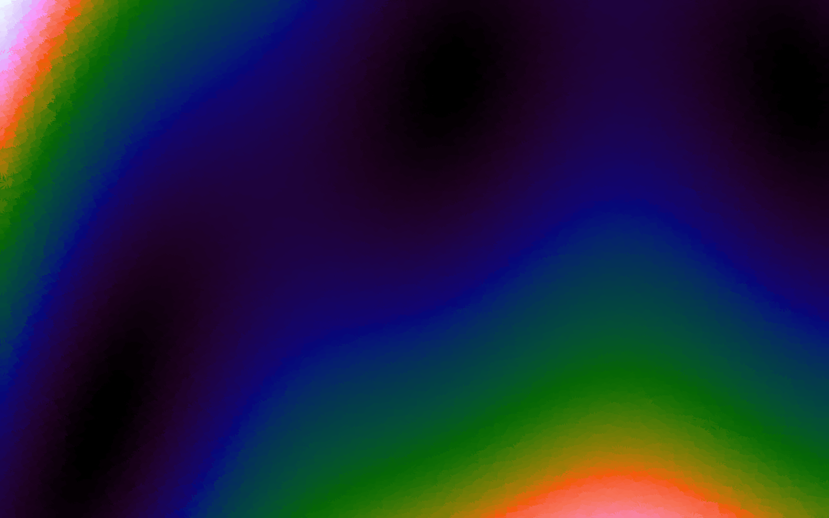
Using the LSH makes it possible to use higher numbers of sample points and do a greater number of queries, as shown in Table 2 below where there are renderings of various sampled functions at 1680 by 1050. The number of samples used was 15,000, taken at random. The number of LSH hashes used was 20 and the bucket size was the diagonal of the function range divided by 1,000. As can be seen, there is some tearing due to the approximate nature of the nearest neighbour search, but because a much greater number of samples can be supported, the function representation is also more accurate.
| Function | Ackley | Branin | Franke's | Goldstein-Price | Sphere |
|---|---|---|---|---|---|
| LSH | 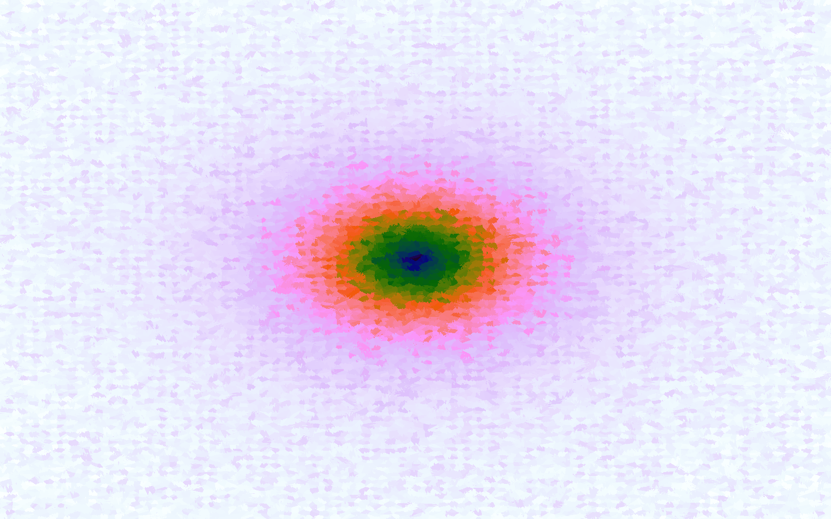 |
 |
 |
 |
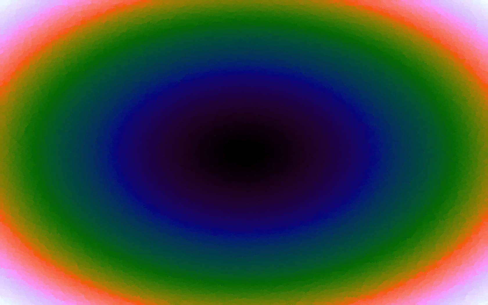 |
Table 2. Approximating functions using LSH to increase the number of sample points.
Interpolation with Inverse Distance Method
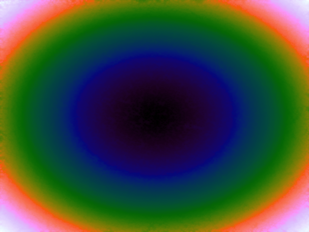
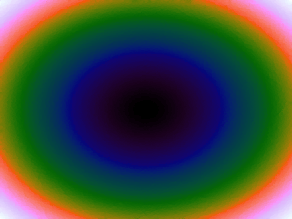
Having more sample points inevitably results in a better approximation, however it might also be possible to better approximate a function using a more sophisticated interpolation method. Although there are several different interpolation methods which can be used for two variables, such as bilinear, an attractive one to use when there is a scattering of points is the inverse distance weighting method, which uses a weighted average based on the distance of the considered sample points from the location of the desired interpolation. The method has a power parameter, p, which determines the relative effect of distance on the weighting of the sample points; the higher, the less effect.
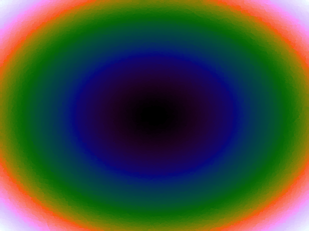
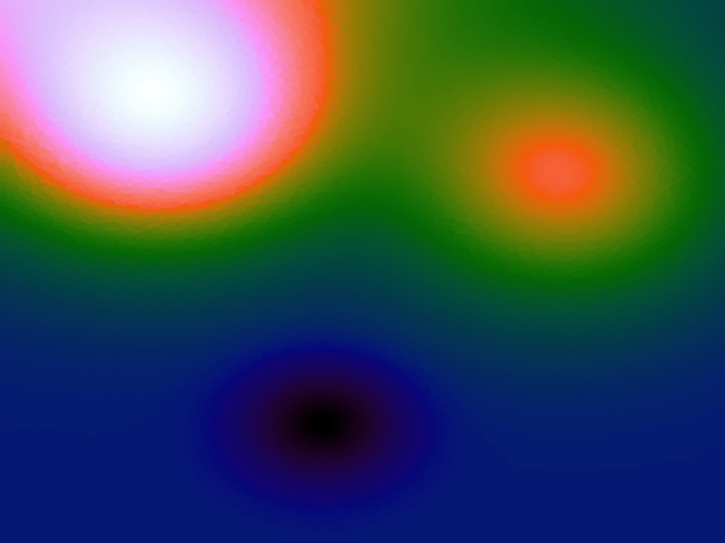
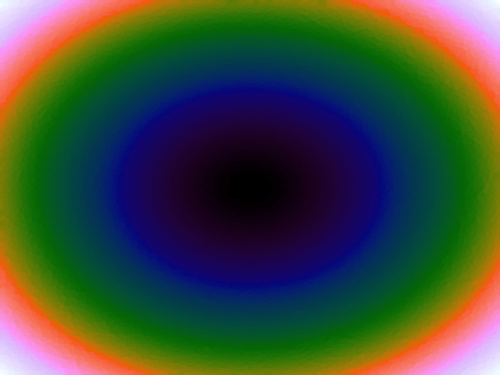
Table 3 below shows the effect of the IDW power parameter on the interpolation. LSH was used with the same parameters as above, but with 20,000 sample points. A value of p = 1 allows a greater effect of more distant points on the interpolated value, creating a fuzzier effect, whereas a p >~ 3 favours the nearest points, pushing it more towards a nearest neighbour interpolation. A power parameter of 2 appears to have the best effect for these functions, although some experimentation might be required for specific applications.
| Function | Ackley | Branin | Franke's | Goldstein-Price | Sphere |
|---|---|---|---|---|---|
| No IDW | 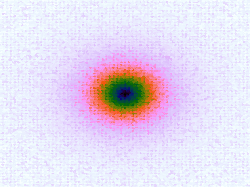 |
 |
 |
 |
 |
| p = 1 | 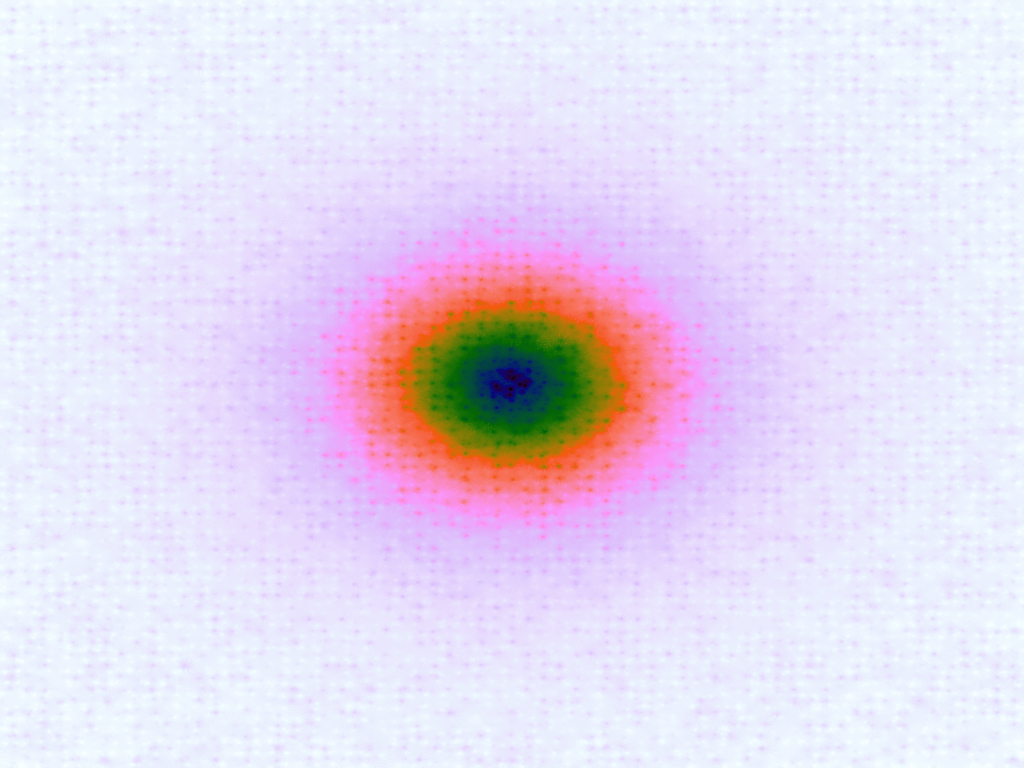 |
 |
 |
 |
 |
| p = 2 | 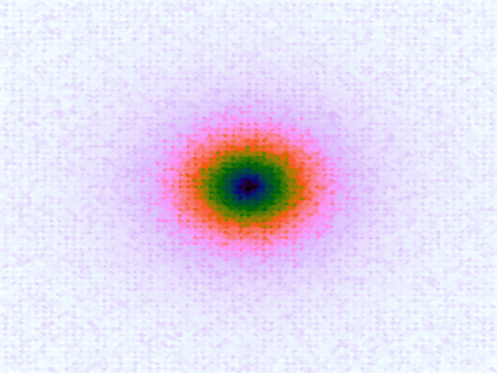 |
 |
 |
 |
 |
| p = 3 | 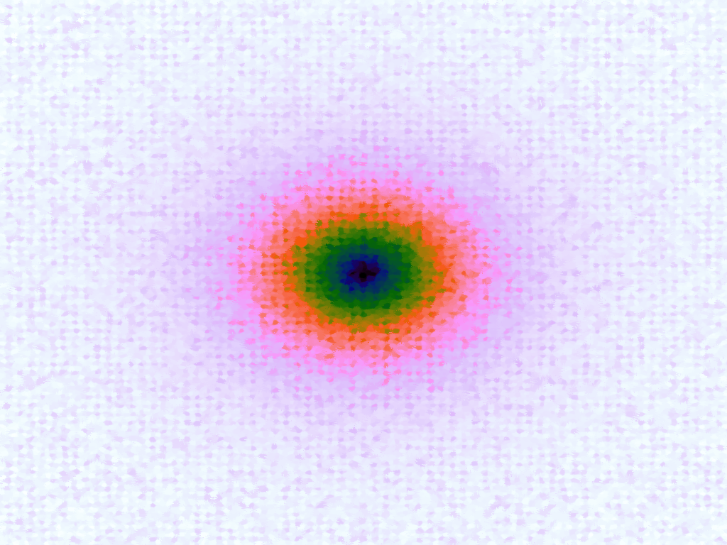 |
 |
 |
 |
 |
| p = 4 | 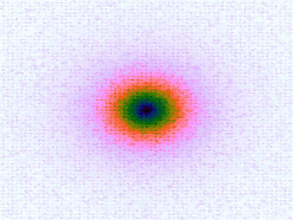 |
 |
 |
 |
 |
Table 3. Comparison of different power parameters for the Inverse Distance Weighting method of interpolation.
use v5.16;

package distance_measures;

sub euclidean_2d {
    my ($p1, $p2) = @_;
    my $d1 = $p2->[0] - $p1->[0];
    my $d2 = $p2->[1] - $p1->[1];
    # omit the square root for speed
    return $d1*$d1 + $d2*$d2;
}

package test_functions;
use Math::Trig;
use List::Util qw( sum0 );

# implement some functions
our %functions = (
    sphere      =>  {
        func        =>      \&sphere_function,
        x_min       =>      -5.12,
        x_max       =>      5.12,
        y_min       =>      -5.12,
        y_max       =>      5.12,
        from        =>      q{https://www.sfu.ca/~ssurjano/spheref.html},
    },

    ackley     =>  {
        func        =>      \&ackley_function,
        x_min       =>      -32.768,
        x_max       =>      32.768,
        y_min       =>      -32.768,
        y_max       =>      32.768,
        from        =>      q{https://www.sfu.ca/~ssurjano/ackley.html},
    },

    frankes     =>  {
        func        =>      \&frankes_function,
        x_min       =>      0,
        x_max       =>      1,
        y_min       =>      0,
        y_max       =>      1,
        from        =>      q{https://www.sfu.ca/~ssurjano/franke2d.html},
    },

    branin     =>  {
        func        =>      \&branin_function,
        x_min       =>      -5,
        x_max       =>      10,
        y_min       =>      0,
        y_max       =>      15,
        from        =>      q{https://www.sfu.ca/~ssurjano/branin.html},
    },

    goldstein_price   =>  {
        func        =>      \&goldstein_price_function,
        x_min       =>      -2,
        x_max       =>      2,
        y_min       =>      -2,
        y_max       =>      2,
        from        =>      q{https://www.sfu.ca/~ssurjano/goldpr.html},
    },
);

sub ackley_function {

    my @x = @_;

    my $a = 20;
    my $b = 0.2;
    my $c = 2*pi;
    my $d = scalar(@x);

    my $p1 = -1 * $b * sqrt(sum0( map { $_*$_ } @x ) / $d);
    my $p2 = sum0( map { cos($c*$_) } @x ) / $d;

    return -1*$a*exp($p1) - exp($p2) + $a + exp(1);
}

sub branin_function {
    my ($x, $y) = @_;

    my $a = 1;
    my $b = 5.1/(4*pi**2);
    my $c = 5/pi;
    my $r = 6;
    my $s = 10;
    my $t = 1/(8*pi);

    my $p1 = $a * ($y - $b*$x**2 + $c*$x - $r)**2;
    my $p2 = $s*(1-$t)*cos($x);

    return $p1 + $p2 + $s;
}

sub frankes_function {
    my ($x, $y) = @_;

    my $p11 = -1.0*((9*$x-2)**2)/4;
    my $p12 = ((9*$y-2)**2)/4;
    my $t1 = 0.75*exp($p11-$p12);

    my $p21 = -1.0*((9*$x+1)**2)/49;
    my $p22 = (9*$y+1)/10;
    my $t2 = 0.75*exp($p21-$p22);

    my $p31 = -1.0*((9*$x-7)**2)/4;
    my $p32 = ((9*$y-3)**2)/4;
    my $t3 = 0.5*exp($p31-$p32);

    my $p41 = -1.0*(9*$x-4)**2;
    my $p42 = (9*$y-7)**2;
    my $t4 = 0.2*exp($p41-$p42);

    return $t1+$t2+$t3-$t4;
}

sub goldstein_price_function {
    my ($x, $y) = @_;

    my $p11 = ($x + $y + 1)**2;
    my $p12 = 19 - 14*$x + 3*$x**2 - 14*$y + 6*$x*$y + 3*$y**2;
    my $p1 = 1 + $p11*$p12;

    my $p21 = (2*$x - 3*$y)**2;
    my $p22 = 18 - 32*$x + 12*$x**2 + 48*$y - 36*$x*$y + 27*$y**2;
    my $p2 = 30 + $p21*$p22;

    return $p1*$p2;
}

sub sphere_function {
    return sum0( map { $_*$_ } @_ );
}

# evaluate the specified function over its default range,
# using its default parameters, to an array of desired dimensions
sub function_2d {

    my ( $func_name, $x_len, $y_len ) = @_;

    # the range over which the function is evaluated
    my ($func_x_s, $func_x_e) = map { $functions{$func_name}{$_} } ('x_min', 'x_max');
    my ($func_y_s, $func_y_e) = map { $functions{$func_name}{$_} } ('y_min', 'y_max');

    # mapping the function range to the desired array dimensions
    my $func_x_dim = $func_x_e - $func_x_s;
    my $func_y_dim = $func_y_e - $func_y_s;

    my $func_x_delta = $func_x_dim / $x_len;
    my $func_y_delta = $func_y_dim / $y_len;

    # evaluate the function over the grid
    my @func_output;
    my $cur_func_y = $func_y_s;
    foreach my $y (0..$y_len-1) {
        my $cur_func_x = $func_x_s;
        foreach my $x (0..$x_len-1) {
            $func_output[$x][$y] = $functions{$func_name}{func}->($cur_func_x, $cur_func_y);
            $cur_func_x += $func_x_delta;
        }
        $cur_func_y += $func_y_delta;
    }

    return \@func_output;
}

package image_stuff;
use Imager;
use Text::CSV;
use List::MoreUtils qw( minmax );

sub write_out {

    my ($fo, $ct, $fname) = @_;

    my $x_dim = scalar(@{$fo});
    my $y_dim = scalar(@{$fo->[0]});

    # flatten the 2D array to 1D
    my @flattened;
    foreach my $y (0..$y_dim-1) {
        foreach my $x (0..$x_dim-1) {
            push @flattened, $fo->[$x][$y];
        }
    }

    # scale for the colour map
    my ($min, $max) = minmax( @flattened );
    my $div = $max - $min;
    die "Divisor is zero" if $div == 0;
    my @scaled_for_img = map { int(255*($_-$min)/$div) } @flattened;

    # create and write a heatmap png image
    my $img = Imager->new(xsize => $x_dim, ysize => $y_dim, channels => 3);
    $img->read( type 				=> 	'raw',
                data 				=> 	pack("C*", map { @{$ct->[$_]} } @scaled_for_img ),
                xsize 				=> 	$x_dim,
                ysize 				=> 	$y_dim,
                raw_datachannels 	=> 	3,
                raw_storechannels 	=> 	3,
                raw_interleave 		=> 	0
                ) or die "Cannot read raw image: ", $img->errstr;

    $img->write( file => "$fname" ) or die $img->errstr;

    return;
}

# read in colour tables from files
sub read_colour_tables {

	my $csv = Text::CSV->new ( { binary => 1 } );

	my %ct;
	my @tables = qw(
		bent-cool-warm-table-byte-0256.csv
		black-body-table-byte-0256.csv
		extended-kindlmann-table-byte-0256.csv
		inferno-table-byte-0256.csv
		kindlmann-table-byte-0256.csv
		plasma-table-byte-0256.csv
		smooth-cool-warm-table-byte-0256.csv
		viridis-table-byte-0256.csv
	);

	foreach my $table (@tables) {

		next unless -e "./colour_tables/" . $table;

		open(my $fh, "<:encoding(utf8)", "./colour_tables/" . $table) or warn "Cannot open $table: $!";
		next unless defined $fh;

		my $table_name = substr( $table, 0, -1 * length("-table-byte-0256.csv") );

		READ_CSV: while ( my $r = $csv->getline( $fh ) ) {
			next READ_CSV unless $r->[1] =~ /\A \d+ \z/ismx;
			push @{ $ct{$table_name} }, [ $r->[1], $r->[2], $r->[3] ];
		}

		close($fh);
	}

	return \%ct;
}

package attractor_map;
use List::Util qw( reduce sum0 );
use List::MoreUtils qw( pairwise );

sub amap_factory {
	my ( $dist_func, $threshold ) = @_;

	$threshold //= 0;
	my %lookup_table;

	return sub {

		my ($input, $output, $new_threshold) = @_;

		$threshold = $new_threshold if defined($new_threshold) && ($new_threshold > 0);

		return undef unless defined($input) && (ref($input) eq 'ARRAY');

		my $input_str = join(",", @{$input});

		$lookup_table{$input_str} = $output if defined $output;

		return $lookup_table{$input_str} if exists $lookup_table{$input_str};	# direct hit!

		my $nearest =
			reduce { $a->[0] < $b->[0] ? $a : $b }
			grep { $_->[0] < $threshold }
			map { [ $dist_func->($_, $input), $_ ] }
			map { [split(/,/, $_)] }
			keys %lookup_table;

		return defined $nearest ? $lookup_table{join(",", @{$nearest->[1]})} : undef;
	}
}

sub amap_LSH_factory {

	my ( $dist_func, $LSH_h, $LSH_l ) = @_;

	my %lookup_table;

    # Setup the LSH.
    my @LSH;    # array of hashes for the LSH, each one has a corresponding random vector.
    # $LSH_h is the number of random vectors to use.
    # $LSH_l is the bucket width.
    # init parameters for the hash key generation functions
    foreach my $i (0..$LSH_h-1) {
        # generate a random vector
        my $v_x = rand(2) - 1;
        my $v_y = rand(2) - 1;
        # for normalisation
        my $mag = sqrt($v_x*$v_x + $v_y*$v_y);
        # the b param is a random offset to move the projection along the "line"
        push @LSH, { vector => [$v_x/$mag, $v_y/$mag], b_param => rand($LSH_l), buckets => {} };
    }

	return sub {

        # multidimensional: expects $input to be an array reference
		my ($input, $output) = @_;

		# be explicit about the result of no input
		return undef unless defined($input) && (ref($input) eq 'ARRAY');

		# stringify the input array for the hash
		my $input_str = join(",", @{$input});

		# if passed an output, then update the lookup table
        if ( defined $output ) {
    		$lookup_table{$input_str} = $output;    # the main lookup table
            # update the locality-sensitive hashes
            foreach my $hash (@LSH) {
                my $projection = $input->[0]*$hash->{vector}[0] + $input->[1]*$hash->{vector}[1];   # projection step
                my $hashkey = int(($projection + $hash->{b_param}) / $LSH_l);                       # bucketing step
                push @{$hash->{buckets}{$hashkey}}, $input;                                         # add the point to the hash bucket
            }
        }

		# performing a lookup
		return $lookup_table{$input_str} if exists $lookup_table{$input_str};	# direct hit!

        # find approximate nearest neigbours using the LSH
        my %ANN;
        foreach my $hash (@LSH) {
            my $projection = $input->[0]*$hash->{vector}[0] + $input->[1]*$hash->{vector}[1];   # projection step
            my $hashkey = int(($projection + $hash->{b_param}) / $LSH_l);                       # bucketing step
            foreach my $nn (@{$hash->{buckets}{$hashkey}}) {                # extract candidate nearest neighbours from the corresponding bucket
                my $pt_str = join(",", @{$nn});
                $ANN{$pt_str} = $lookup_table{$pt_str};                                    # add them to the list. This will dedupe if necessary
            }
        }

        # scalar(keys %ANN) should be significantly smaller than scalar(keys %lookup_table) and
        # have a high probability of containing the nearest neighbour if $LSH_h is big enough.

        # find the nearest out of that subset
		my $nearest =						         # 5. $nearest = [ distance, vector ]
			reduce { $a->[0] < $b->[0] ? $a : $b }   # 4. find the closest (minimum) out of those
			map { [ $dist_func->($_, $input), $_ ] } # 3. compute distance from input vector, put beside original vector
			map { [split(/,/, $_)] }                 # 2. un-stringify to vector
			keys %ANN;				                 # 1. for all (approximate) nearest neighbours from LSH

        # have to re-stringify to perform lookup.
		return defined $nearest ? $lookup_table{join(",", @{$nearest->[1]})} : undef;
	}
}

sub amap_LSH_IDW_factory {

	my ( $dist_func, $LSH_h, $LSH_l, $p ) = @_;

	my %lookup_table;
    $p //= 2;               # p is the power parameter for the IDW

    # Setup the LSH.
    my @LSH;    # array of hashes for the LSH, each one has a corresponding random vector.
    # $LSH_h is the number of random vectors to use.
    # $LSH_l is the bucket width.
    # init parameters for the hash key generation functions
    foreach my $i (0..$LSH_h-1) {
        # generate a random vector
        my $v_x = rand(2) - 1;
        my $v_y = rand(2) - 1;
        # for normalisation
        my $mag = sqrt($v_x*$v_x + $v_y*$v_y);
        # the b param is a random offset to move the projection along the "line"
        push @LSH, { vector => [$v_x/$mag, $v_y/$mag], b_param => rand($LSH_l), buckets => {} };
    }

	return sub {

        # multidimensional: expects $input to be an array reference
		my ($input, $output) = @_;

		# be explicit about the result of no input
		return undef unless defined($input) && (ref($input) eq 'ARRAY');

		# stringify the input array for the hash
		my $input_str = join(",", @{$input});

		# if passed an output, then update the lookup table
        if ( defined $output ) {
    		$lookup_table{$input_str} = $output;    # the main lookup table
            # update the locality-sensitive hashes
            foreach my $hash (@LSH) {
                my $projection = $input->[0]*$hash->{vector}[0] + $input->[1]*$hash->{vector}[1];   # projection step
                my $hashkey = int(($projection + $hash->{b_param}) / $LSH_l);                       # bucketing step
                push @{$hash->{buckets}{$hashkey}}, $input;                                         # add the point to the hash bucket
            }
        }

		# performing a lookup
		return $lookup_table{$input_str} if exists $lookup_table{$input_str};	# direct hit!

        # find approximate nearest neigbours using the LSH
        my %ANN;
        foreach my $hash (@LSH) {
            my $projection = $input->[0]*$hash->{vector}[0] + $input->[1]*$hash->{vector}[1];   # projection step
            my $hashkey = int(($projection + $hash->{b_param}) / $LSH_l);                       # bucketing step
            foreach my $nn (@{$hash->{buckets}{$hashkey}}) {                # extract candidate nearest neighbours from the corresponding bucket
                my $pt_str = join(",", @{$nn});
                $ANN{$pt_str} = $lookup_table{$pt_str};                                    # add them to the list. This will dedupe if necessary
            }
        }

        # scalar(keys %ANN) should be significantly smaller than scalar(keys %lookup_table) and
        # have a high probability of containing the nearest neighbour if $LSH_h is big enough.
        # Use IDW to get a weighted average for the output value

        my @IDW_keys = keys %ANN;
        my @IDW_vals = values %ANN;

        my @weights =
            map { 1/$dist_func->($_, $input)**$p; }
            map { [split(/,/, $_)] }
            @IDW_keys;

        my $denominator = sum0 ( @weights );

        if ( $denominator == 0 ) {
            warn "Denominator is 0";
        }

        return sum0( pairwise { $a*$b } @IDW_vals, @weights ) / $denominator;
	}
}

sub amap_IDW_factory {

	my ( $dist_func, $p ) = @_;

	my %lookup_table;
    $p //= 2;               # p is the power parameter for the IDW

	return sub {

        # multidimensional: expects $input to be an array reference
		my ($input, $output) = @_;

		# be explicit about the result of no input
		return undef unless defined($input) && (ref($input) eq 'ARRAY');

		# stringify the input array for the hash
		my $input_str = join(",", @{$input});

		# if passed an output, then update the lookup table
		$lookup_table{$input_str} = $output if defined $output;

		# performing a lookup
		return $lookup_table{$input_str} if exists $lookup_table{$input_str};	# direct hit!

        # If not a direct hit, use inverse distance weighting to get a
        # weighted average for the output point
        # https://en.wikipedia.org/wiki/Inverse_distance_weighting
        my @IDW_keys = keys %lookup_table;
        my @IDW_vals = values %lookup_table;

        my @weights =
            map { 1/$_**$p; }
            map { $dist_func->($_, $input) }
            map { [split(/,/, $_)] }
            @IDW_keys;

        my $denominator = sum0 ( @weights );

        if ( $denominator == 0 ) {
            warn "Denominator is 0";
            return undef;
        }

        return sum0( pairwise { $a*$b } @IDW_vals, @weights ) / $denominator;
	}
}

package main;
use MCE::Stream;

my $img_x_dim = 1024;
my $img_y_dim = 768;

# read the colour tables
my $colour_tables = image_stuff::read_colour_tables();
my $cmap = "extended-kindlmann";
my @ct_to_use = @{ $colour_tables->{$cmap} };

foreach my $func_name (keys %test_functions::functions) {

    # get range
    my ($func_x_s, $func_x_e) = map { $test_functions::functions{$func_name}{$_} } ('x_min', 'x_max');
    my ($func_y_s, $func_y_e) = map { $test_functions::functions{$func_name}{$_} } ('y_min', 'y_max');

    my $func_x_dim = $func_x_e - $func_x_s;
    my $func_y_dim = $func_y_e - $func_y_s;

    # pre-compute the function x,y coords for each x,y coord in the output array
    my $func_x_delta = $func_x_dim / $img_x_dim;
    my $func_y_delta = $func_y_dim / $img_y_dim;

    my @x_vals = map { $func_x_s + $func_x_delta*$_} (0..$img_x_dim-1);
    my @y_vals = map { $func_y_s + $func_y_delta*$_} (0..$img_y_dim-1);

    # number of points to seed
    my $points = 20000;

    # have an attempt to calculate LSH bucket sizes
    my $LSH_l_1000 = sqrt($func_x_dim**2 + $func_y_dim**2) / 1000;

    my %amaps = (
        amap                    =>      attractor_map::amap_factory( \&distance_measures::euclidean_2d, 1000 ),
        amap_IDW_p2             =>      attractor_map::amap_IDW_factory( \&distance_measures::euclidean_2d, 2 ),
        amap_LSH_l1000          =>      attractor_map::amap_LSH_factory( \&distance_measures::euclidean_2d, 20, $LSH_l_1000 ),
        amap_LSH_l1000_IDW_p1   =>      attractor_map::amap_LSH_IDW_factory( \&distance_measures::euclidean_2d, 20, $LSH_l_1000, 1 ),
        amap_LSH_l1000_IDW_p2   =>      attractor_map::amap_LSH_IDW_factory( \&distance_measures::euclidean_2d, 20, $LSH_l_1000, 2 ),
        amap_LSH_l1000_IDW_p3   =>      attractor_map::amap_LSH_IDW_factory( \&distance_measures::euclidean_2d, 20, $LSH_l_1000, 3 ),
        amap_LSH_l1000_IDW_p4   =>      attractor_map::amap_LSH_IDW_factory( \&distance_measures::euclidean_2d, 20, $LSH_l_1000, 4 ),
            );

    # add random data points to the attractor maps
    foreach my $count_inner (0..$points) {

        my $rand_x = $func_x_s + rand($func_x_dim);
        my $rand_y = $func_y_s + rand($func_y_dim);

        foreach my $func (values %amaps) {
            $func->([$rand_x, $rand_y], $test_functions::functions{$func_name}{func}->($rand_x, $rand_y));
        }
    }

    # query the attractor maps to get values for all the coords.
    foreach my $amap_name (keys %amaps) {

        # use the Perl MCE to get a parallel processing speedup
        my @func_output;
        mce_stream \@func_output,
                    sub {
                        my @m1;
                        foreach my $y (@y_vals) {
                            push @m1, $amaps{$amap_name}->([$_, $y]);
                        }
                        return \@m1;
                    },
                    @x_vals;

        # write it out as an image
        my $filename = join("_", $func_name, $amap_name, $points, $img_x_dim . "x" . $img_y_dim, $cmap) . ".png";
        image_stuff::write_out( \@func_output, \@ct_to_use, $filename );
    }
}

exit;